cartography in R part four

Welcome to part four of my cartography in R series. In this post, we’ll download and process the state park data before adding it to the base map created in part II.

project outline

I had to break the tutorial into different parts because it became unwieldy. I list the component parts below. The annotated version of the code can be found in this project’s repository in the folder called r files

I. cartography in r part one

• install packages
• download usa shapefile
• shift alaska and hawaii
• save shapefile

II. cartography in r part two

• create usa base map

III. cartography in r part three

• download national park data
• process national park data
• shift alaska and hawaii national parks
• save shapefile
• add national parks to map

IV. cartography in r part four

• download state park data
• process state park data
• shift alaska and hawaii state parks
• separate state park data
• save state park data

V. cartography in r part five

• add in shiny functionality
• add markers to visited parks
• save and embed map

VI. cartography in r part six

• create individual state maps
• add in shiny functionality
• add markers to visited parks
• save and embed maps

1. load libraries

1
2
3
4
5
    ## load libraries
    library("tidyverse")        # data manipulation & map creation
    library("sf")               # loads shapefile
    library("leaflet")          # creates the map
    library("operator.tools")   # not-in function

I am not going to explain in detail what each of these packages do because I already covered it in part one.

2. load data

1
2
3
    ## load data
    usa <- read_sf("~/Documents/Github/nps/shapefiles/shifted/usa/usa.shp")
    nps <- read_sf("~/Documents/GitHub/nps/shapefiles/shifted/nps/nps.shp")

Be sure to change ~/Documents/Github/nps/shapefiles/shifted/usa/usa.shp and ~/Documents/GitHub/nps/shapefiles/shifted/nps/nps.shp to reflect where you saved the shifted shapefiles.

If your data processing and base map creation are in the same file, you can skip these lines. When you make the Leaflet call below, you’ll use the name of the variable where the shape data is stored.

3. download state park data

Unlike the National Park data, the state data is harder to come by. After quite a bit of searching I found the Protected Areas Database of the United States (PAD-US) created by the United States Geological Survey. The data they collect is amazing. It is a “national inventory of U.S. terrestrial and marine protected areas.”

When they say national inventory, they mean it. It includes a detailed accounting of nearly every piece of public land “preserved through legal or other effective means” in the United States. For my project, it’s overkill and it will take some investigating to determine what information I want to keep and what to discard.

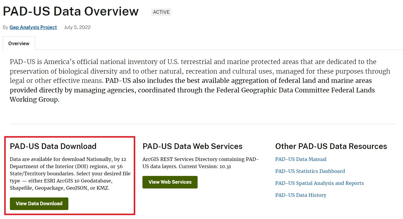
The first step is to navigate to the PAD-US website and download the data. On the PAD-US website, click View Data Download.

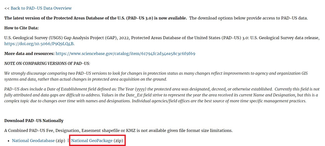
On the next page, you can download the National PAD-US data, the data by Census region, and by state. Click on National Geopackage. Make sure you select the geopackage one rather than the geodatabase version. On the next page, you’ll confirm you’re not a robot before the download link appears.

When it downloads, unzip it somewhere on your hard drive. The zip folder contains 35 files, so I suggest you create a folder before unzipping it so they stay together.

4. find the right layer

Since the geopackage is so large, R has a difficult time opening and displaying the data. There’s a couple of ways to view the data that does not rely on R. First, is to load the geopackage layers. This doesn’t load the complete data set. Instead, it just loads the layer names to use in conjunction with the documentation and the PAD-US Viewer.

1
    layers <- st_layers("./shapefiles/original/state parks/padus_national_gpkg/PADUS3_0Geopackage.gpkg")

I save the layer names to a variable called layers so I can load them whenever I want. You don’t have to, the st_layers() function will return the list regardless of whether it’s saved.

st_layers() returns the name of the layer, then what kind of layer it is (Multi Polygon), how many features it contains, and what coordinate system it uses.

The PAD-US geopackage contains seven layers which contain different kinds of information. The type of map you want to create will determine which layer you will use. For my map I want the same information for the state parks as I have for the national parks. I want:

• the state where the park is located
• the park name
• the park type
• and the park’s size.

I have to figure out which of the seven layers listed above includes this information. You can load each layer (using the st_read() code below), but this method usually causes R to crash because there’s too much information for it to handle.

Instead, I go to the PAD-US Viewer and search for a state park. I am going to choose the Valley of Fire State Park in Nevada because 1) I know it exists, 2) I have been there. You can choose any state park you’ve been to, or choose one from a list of parks by state on Wikipedia.

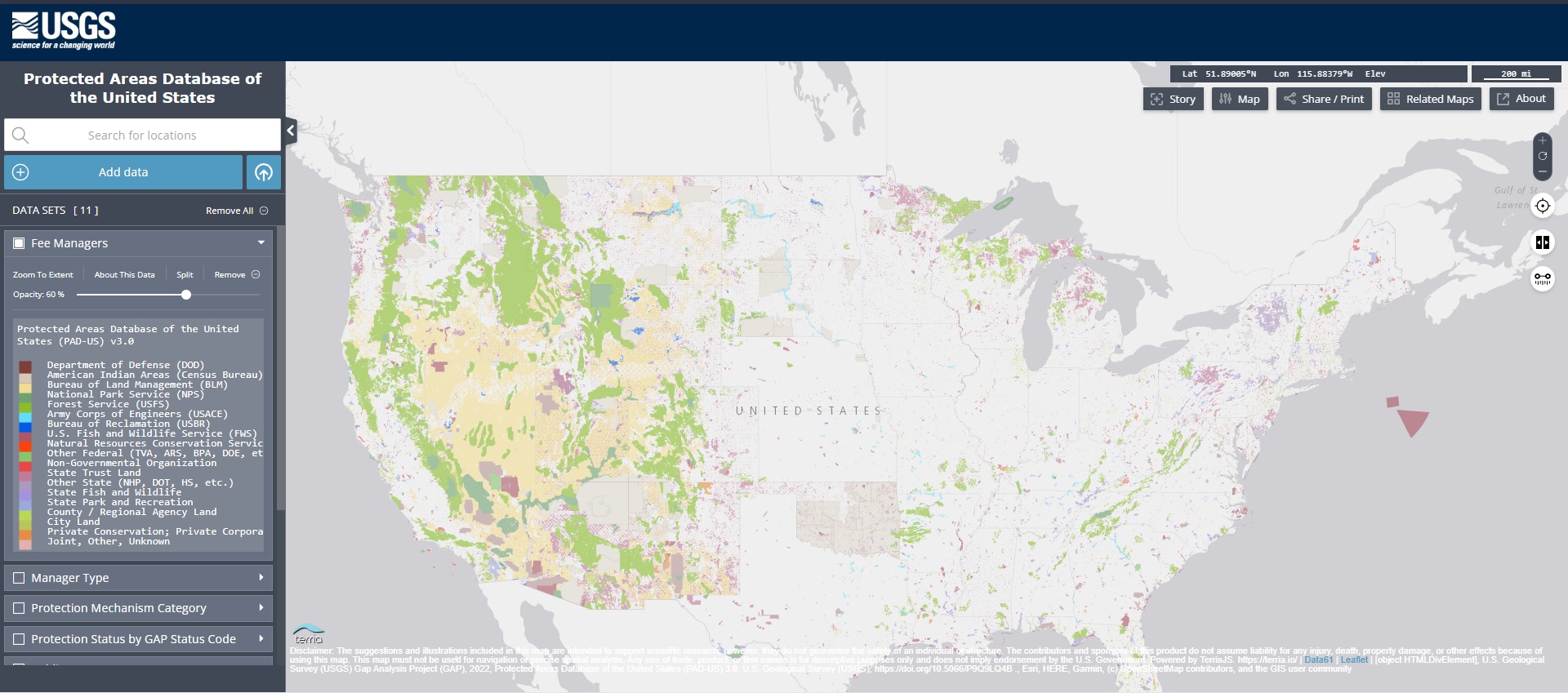
In the search bar on the left, (1) type in Valley of Fire, (2) select it from under the Official Place Names panel that appears after you start typing, the map will adjust to show the park and (3) you can click Done

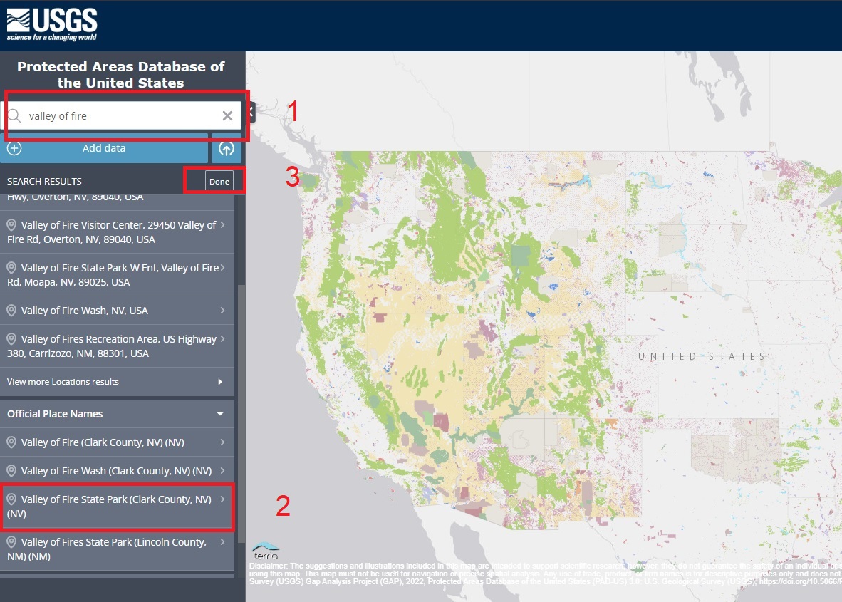
The default view on the PAD-US Viewer includes the first layer’s information, Fee Managers in the viewer and PADUS3_0Fee in the geopackage. According to the documentation, most public land is “owned in fee” though some land is held in “long-term easements, leases, agreements” or by Congressional designation. To own land “in fee” means to own it completely, without limitations or conditions. The Fee layer lists what agency owns the land in its entirety.

I don’t actually care whether it’s in fee or easement (allowed to use someone else’s land), my interest is solely in whether the Park’s polygon is visible when this layer is selected in the viewer.

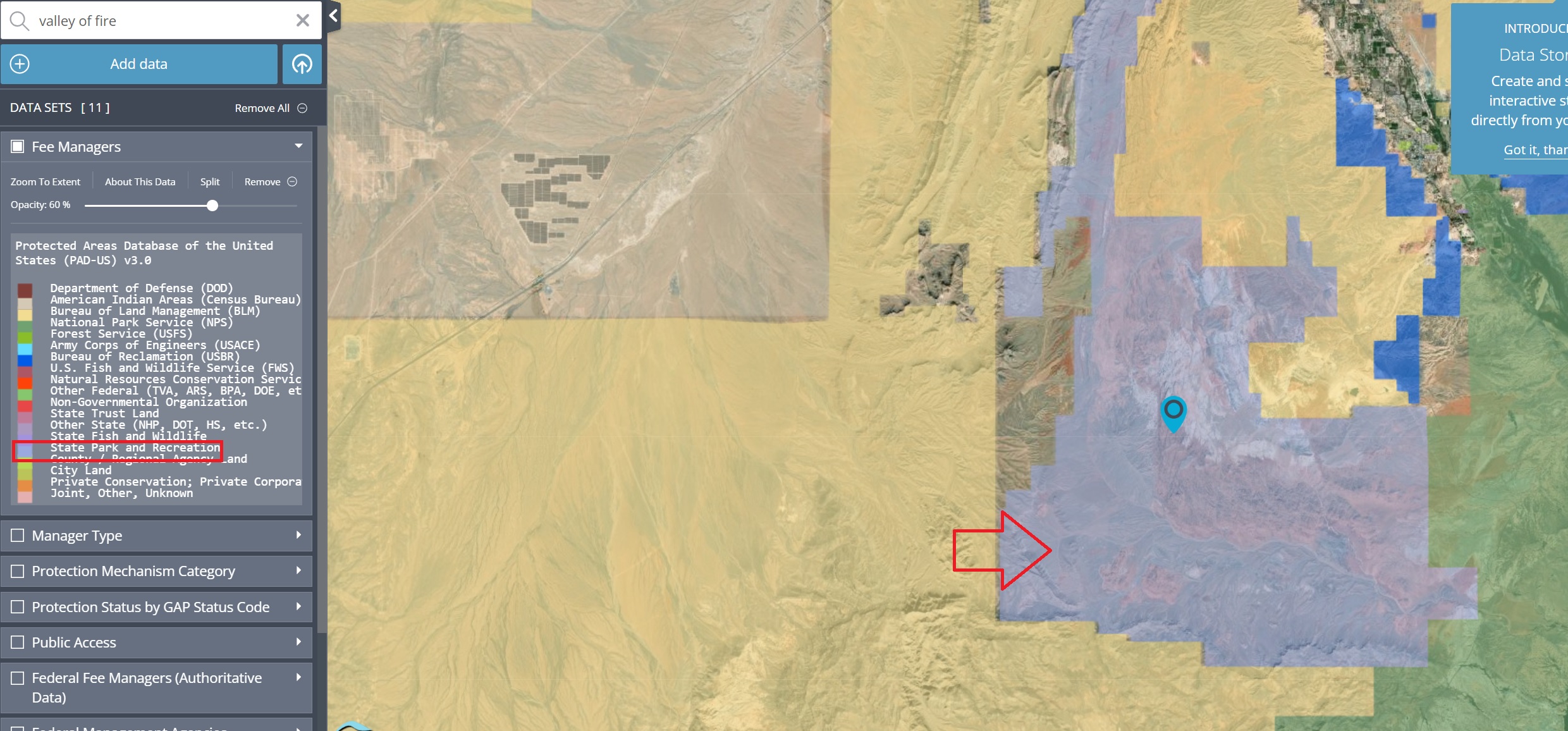
The purple-ish polygon on the map shows the geographic boundaries of the Valley of Fire State Park. This is what I want to see. Not all of the layers include the shape data for the state parks.

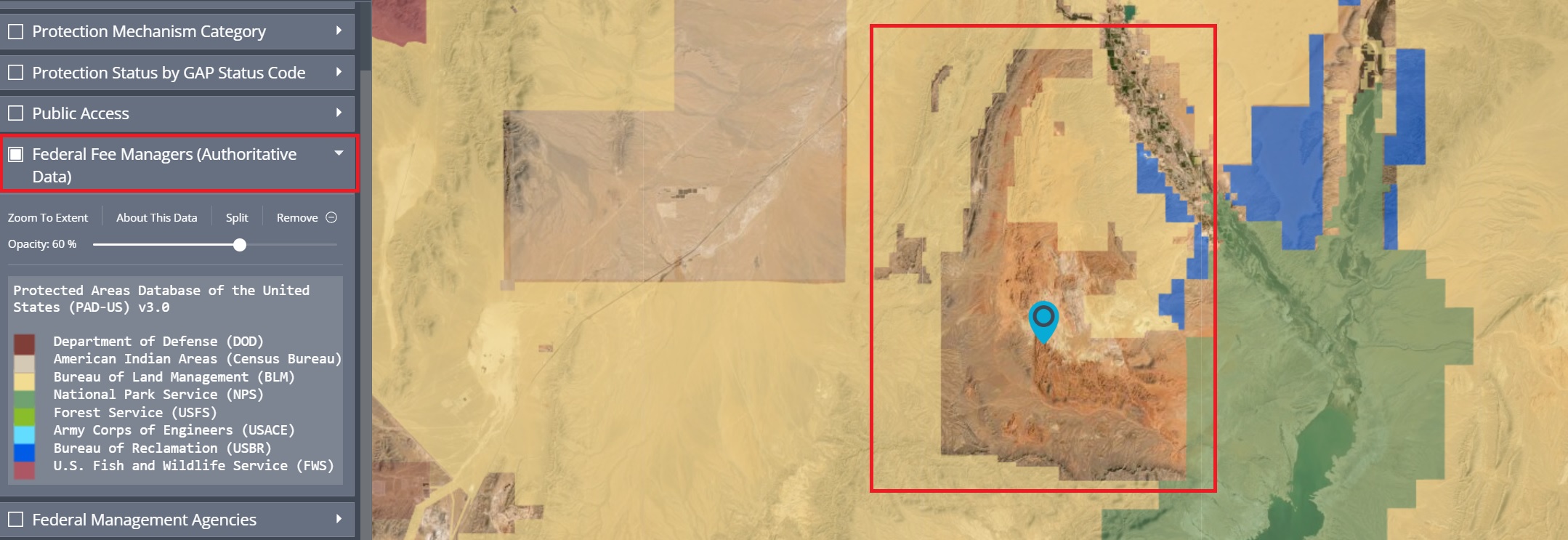
For example, if I uncheck the Fee Manager layer and select the Federal Fee Managers (Authoritative Data) layer the polygon for the Valley of Fire disappears. This is because the Valley of Fire is not federal land - it’s state land. Be careful when choosing the layers because not all of them contain the correct information.

5. find the right data

The USGS is interested in fundamentally different information than I am. Finding the right information for my map is going to take some data manipulation. Since the USGS is interested in the more technical aspects of land management, their categories are more detailed than what I need.

Using the PAD-US Viewer, I can investigate what information is available without having to load the entire data set into R’s viewer.

For this section, I am going to use the Valley of Fire State Park in Nevada, Crissey Field State Recreation Site in Oregon, and the Salton Sea State Recreation Area in California to make sure that I am getting the data I want from the Fee layer. I chose these parks because I have been to them. I know where they are and that they are all (mostly) state land.

First, I need a good way to filter out national, tribal, or military land. On the PAD-US Viewer I will look at the Valley of Fire State Park information. When you search for it (described above) a marker will pop up. If you click on the marker a table will show on the map that includes all the information available on that layer.

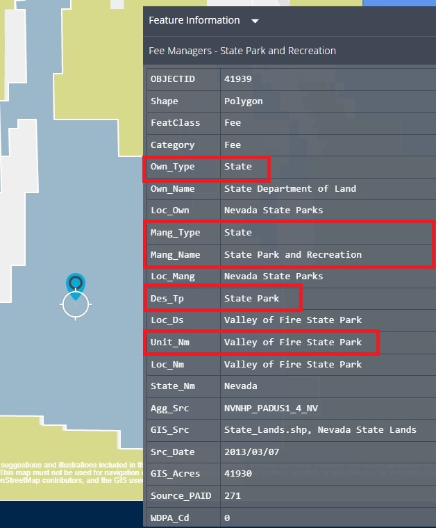
In the image the values on the left are the variable names - I’ll use these later to select certain variables. On the right is the value for the specific park. I’ve boxed a few of the properties which I’ll check across the different parks to make sure I can get all the information I need.

1. Own_Type designates who owns the land. For Valley of Fire it’s state owned land.
2. Mang_Type is the name of the agency that manages the land.
3. Mang_Name is the type of agency that owns the land.
4. Des_Tp is the designation type.
5. Unit_Nm is the land’s name.

When we look at Crissey Field, many of these fields have different values.

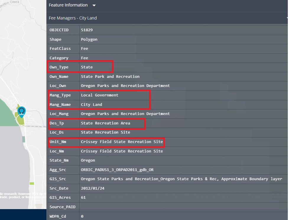
The ownership type (Own_Type) is the same for both: State. The Mang_Type, Mang_Name, Des_Tp, and (obviously) Unit_Nm are different.

Next, we need to check the Salton Sea. The Salton Sea demonstrates the problem with finding appropriate data. Since the Salton Sea is toxic, it’s owned in part by the State of California, the Bureau of Land Management, and the Bureau of Reclamation - each represented by a different color on the map.

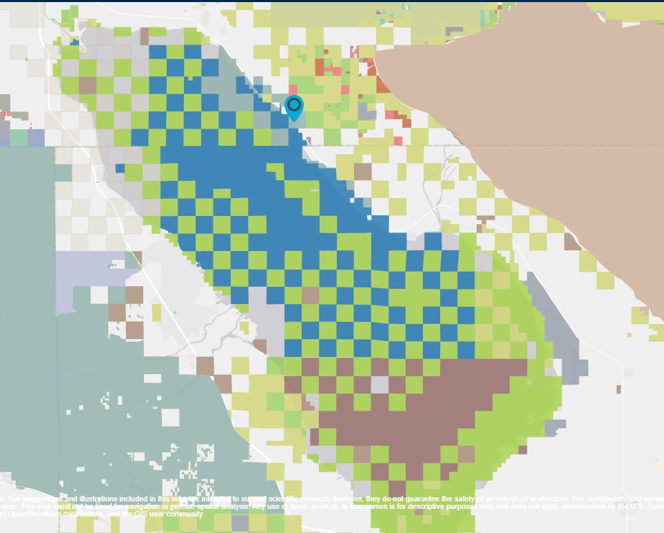
Having visited the park, I can tell you there’s no fences or markers designating the different owners. On paper the Salton Sea may have many different owners, in real life you wouldn’t know it just by visiting the area.

On the left hand side of the viewer there’s a color-coded key that indicates the different Fee managers. It’s not very user-friendly because the the colors are very similar.

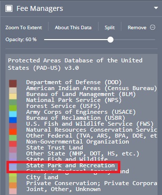
I don’t actually care who the fee manager of the Salton Sea is. What I am looking for, though, is whether any part of the Salton Sea includes Own_Type as State. If it does, I can use this column to separate the state data from any other kind.

In the viewer, I’ll look for the blueish violet color (boxed in red above).

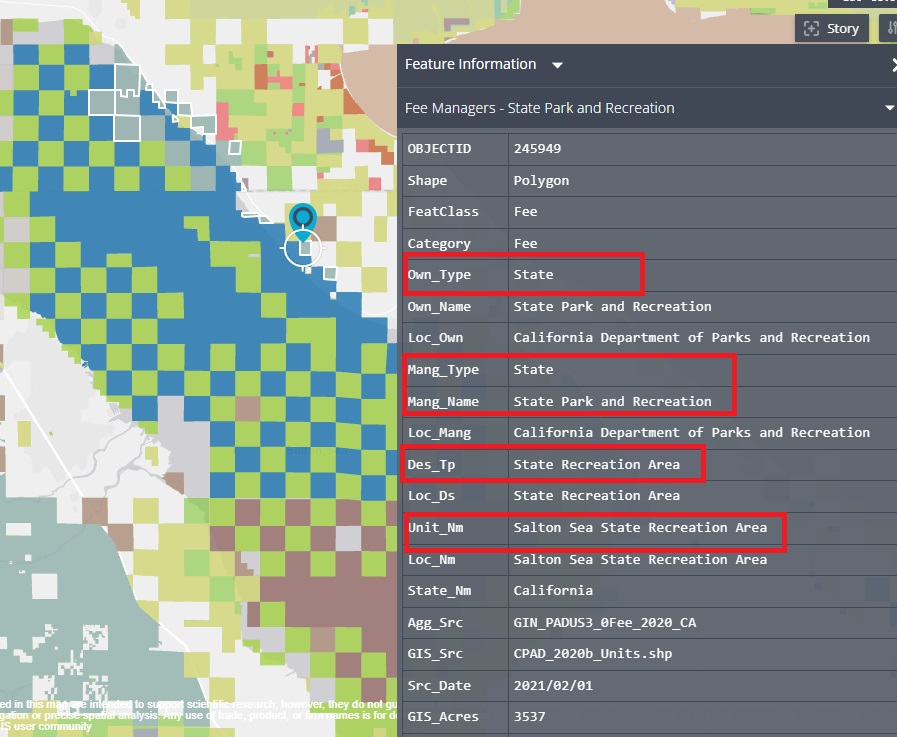
After some trial and error I found a location about a quarter of the way down the lake’s right hand side. I am fairly certain I’ve actually been to that exact location. When looking at the table, I can see that the Own_Type matches the Valley of Fire and Crissey Fields which means I can select the state data using this property.

Now we’ll move back to R to load the data layer, filter for the 50 states, and for state owned land.

6. process state park data

1
2
3
4
5
6
7
8
9
10
11
12
13
14
15
16
17
18
19
20
21
22
23
24
25
26
27
28
29
30
31
32
33
34
35
36
37
38
39
40
41
42
43
    ## create territories list
    territories <- c("AS", "GU", "MP", "PR", "VI")

    state_parks <- st_read("./shapefiles/original/state_parks_padus/PADUS3_0Geopackage.gpkg", layer = "PADUS3_0Fee")  %>%
    filter(State_Nm %!in% territories & 
           Own_Type == "STAT")  %>% 
    filter(Des_Tp == "ACC" |
           Des_Tp == "HCA" |
           Des_Tp == "REC" |
           Des_Tp == "SCA" |
           Des_Tp == "SHCA" |
           Des_Tp == "SP" |
           Des_Tp == "SREC" |
           Des_Tp == "SRMA" |
           Des_Tp == "SW") %>% 
    filter(d_Pub_Acce != "Closed" & 
           d_Pub_Acce != "Unknown") %>% 
    filter(Loc_Ds != "ACC" &
           Loc_Ds != "Hunter Access",
           Loc_Ds != "Public Boat Ramp")  %>% 
    select(d_Own_Type, d_Des_Tp, Loc_Ds, Unit_Nm, State_Nm, d_State_Nm, GIS_Acres)  %>% 
    mutate(type = case_when(d_Des_Tp == "Access Area" ~ "State Trail",
                            d_Des_Tp == "Historic or Cultural Area" ~ "State Historical Park, Site, Monument, or Memorial",
                            d_Des_Tp == "State Historic or Cultural Area" ~ "State Historical Park, Site, Monument, or Memorial",
                            d_Des_Tp == "Recreation Management Area" ~ "State Preserve, Reserve, or Recreation Area",
                            d_Des_Tp == "State Resource Management Area" ~ "State Preserve, Reserve, or Recreation Area",
                            d_Des_Tp == "State Wilderness" ~ "State Preserve, Reserve, or Recreation Area",
                            d_Des_Tp == "State Recreation Area" ~ "State Preserve, Reserve, or Recreation Area",
                            d_Des_Tp == "State Conservation Area" ~ "State Preserve, Reserve, or Recreation Area",
                            d_Des_Tp == "State Park" ~ "State Park or Parkway"))  %>% 
    mutate(visited = case_when(Unit_Nm == "Valley of Fire State Park" ~ "visited",
                               Unit_Nm == "Crissey Field State Recreation Site" ~ "visited",
                               Unit_Nm == "Salton Sea" ~ "visited",
                               Unit_Nm == "Anza-Borrego Desert State Park" ~ "visited",
                               Unit_Nm == "Jedediah Smith Redwoods State Park" ~ "visited",
                               Unit_Nm == "Del Norte Coast Redwoods State Park" ~ "visited",
                               TRUE ~ "not visited")  %>% 
    shift_geometry(preserve_area = FALSE, 
                    position = "below") %>% 
    sf::st_transform("+proj=longlat +ellps=WGS84 +datum=WGS84 +no_defs")

    ## save shifted park data
    # st_write(state_parks, "./shapefiles/shifted/states/state_parks.shp")

These lines should be familiar by now, so I will briefly cover them here. For a detailed description of each line, check out part III of this series.

• line 2

2    territories <- c("AS", "GU", "MP", "PR", "VI")

Line 2 creates the list of US territories that I filter out in line 5.

If you want to read more about this line visit part III of the series.

• line 4

4    state_parks <- st_read("./shapefiles/original/state_parks_padus/PADUS3_0Geopackage.gpkg", layer = "PADUS3_0Fee")  %>%

Since we’re working with a geopackage (instead of a shapefile) we have to load the data using st_read() instead of read_sf()

st_read() takes two arguments. The first is the path to the geopackage. When we downloaded the PAD-US data and unzipped it, the folder contained 35 files. From those 35 make sure you choose the one with the .gpkg extension.

The second argument layer = specifies which layer R should load. Here, I am selecting the layer PADUS3_0Fee layer because I know it contains the shape data from the state parks.

• lines 5-6

5    filter(State_Nm %!in% territories  &
6           Own_Type == "STAT")

R and the Tidyverse’s filter() function allows you to combine conditions within one filter call by using and (&) OR or (|).

The logic in this line says filter the data for rows where the State_Nm is not in %!in% the territories list (discard all but the 50 states) and (&) the Own_Type is (==) STAT. For the row to be selected, both conditions must evaluate to true. This will keep only state parks from the 50 states.

The original unfiltered data set had 247,507 rows. After these the two conditions are met, the filtered data set has 53,139 rows. That’s a significant reduction but still a substantial number of rows.

• lines 7-15

7    filter(Des_Tp == "ACC" |
8           Des_Tp == "HCA" |
9           Des_Tp == "REC" |
10          Des_Tp == "SCA" |
11          Des_Tp == "SHCA" |
12          Des_Tp == "SP" |
13          Des_Tp == "SREC" |
14          Des_Tp == "SRMA" |
15          Des_Tp == "SW")  

Theoretically, lines 7-15 can be included with the first filter() call in line 5, but I couldn’t get it to work.

Next, I want to choose certain types of state owned land. For that, I am going to look at the Des_Tp column. According to the PAD-US documentation, the Des_Tp column holds information about the Designation Type. It contains 37 different land designations.

I am going to restrict my data to include the following designations:

• ACC (Access Areas) - after much searching this includes Hunter Access areas, Boat Ramps, and Trails. I’m most interested in the Trails.
• HCA (Historic or Cultural Area)
• REC (Recreation Management Area)
• SCA (State Conservation Area)
• SHCA (State Historical or Cultural Area)
• SP (State Park)
• SREC (State Recreation Area)
• SRMA (State Recreation Management Area)
• SW (State Wilderness)

This will leave me with 50,102 rows.

• Lines 16-17

16    filter(d_Pub_Acce != "Closed" & 
17           d_Pub_Acce != "Unknown")  %>% 

Yet another filter() call. These two lines tell R to exclude any row whose d_Pub_Acce is not Closed or Unknown

The data has four types of access: Closed, Unknown, Open Access, and Restricted Access. I’m only interested in land that I can visit, so I want to keep only the parks with Open or Restricted Access. In the filter() call, I chose to use != solely because months or years from now when I look at this code it will be easier for me to figure out what I was doing. I know myself and if I saw d_Pub_Acce == "Open Access" my first thought would be: “What are the other types?” and then I’ll try and find out and waste a bunch of time.

This last filter brings the total number of state parks down to 49,719. I don’t think I can reduce that number more without removing places that should be kept.

• lines 18-20

18    filter(Loc_Ds != "ACC" &
19           Loc_Ds != "Hunter Access",
20           Loc_Ds != "Public Boat Ramp")

Lines 18-20 have the same logic as lines 16-17 except here I want to filter out the Hunter Access areas and Boat Ramps.

• Line 21

21      select(d_Own_Type, d_Des_Tp, Loc_Ds, Unit_Nm, State_Nm, d_State_Nm, GIS_Acres, SHAPE)  %>% 

Now that I’ve pared down the data a little bit, I want discard any column don’t need.

select() lets me choose the columns I want to keep by name, rather than by index number.

I decided to keep:

• d_Own_Type (owner type)
• d_Des_Tp (designation type - state park, resource area, etc)
• Loc_Ds (location description - I like this because it tells me where ponds are)
• Unit_Nm (park name)
• State_Nm (two character state abbreviation)
• d_State_Nm (long state name)
• GIS_Acres (park size)
• SHAPE (geometry column)

• lines 22-30

22  mutate(type = case_when(d_Des_Tp == "Access Area" ~ "State Trail",
23                          d_Des_Tp == "Historic or Cultural Area" ~ "State Historical Park, Site, Monument, or Memorial",
24                          d_Des_Tp == "State Historic or Cultural Area" ~ "State Historical Park, Site, Monument, or Memorial",
25                          d_Des_Tp == "Recreation Management Area" ~ "State Preserve, Reserve, or Recreation Area",
26                          d_Des_Tp == "State Resource Management Area" ~ "State Preserve, Reserve, or Recreation Area",
27                          d_Des_Tp == "State Wilderness" ~ "State Preserve, Reserve, or Recreation Area",
28                          d_Des_Tp == "State Recreation Area" ~ "State Preserve, Reserve, or Recreation Area",
29                          d_Des_Tp == "State Conservation Area" ~ "State Preserve, Reserve, or Recreation Area",
30                          d_Des_Tp == "State Park" ~ "State Park or Parkway"))

mutate() is part of the tidyverse package and it’s extremely versatile. It is mainly used to create new variables or modify existing ones.

I wanted the state park designations to match closely with the types I used in the National Park data.

I went over the logic of using mutate() and case_when() in Part III of this series, so I won’t cover it again here.

In its general form, the format is case_when(COLUMN_NAME == "original_value" ~ "new_value"). I only needed to change the values for any "Recreation Management Area", the rest I just populated the new column with the old values.

• lines 31-37

31  mutate(visited = case_when(Unit_Nm == "Valley of Fire State Park" ~ "visited",
32                             Unit_Nm == "Crissey Field State Recreation Site" ~ "visited",
33                             Unit_Nm == "Salton Sea" ~ "visited",
34                             Unit_Nm == "Anza-Borrego Desert State Park" ~ "visited",
35                             Unit_Nm == "Jedediah Smith Redwoods State Park" ~ "visited",
36                             Unit_Nm == "Del Norte Coast Redwoods State Park" ~ "visited",
37                             TRUE ~ "not visited")  %>% 

Here is where I ran into some issues. In part III of the series when I processed the National Park data I included a mutate() and case_when() call to mark whether I’ve visited the park or not. It’s not a very elegant solution since I have to modify each park individually, but it was passable since I’ve only been to a handful of National Parks. For the state parks, though, it is unwieldy.

I had original wanted to drop the geometry and download the parks as a CSV, edit it using Excel or LibreCalc, then load and merge it with the geometry data, but even that was overwhelming. With approximately 50,000 rows it was a very large file. I know I could filter out states I haven’t visited to get than number down, but since I live in California there are still a lot of parks to get through.

In the end, I decided to focus on the parks that I know I’ve visited and have taken photos at. I’ve visited many, many state parks, but until I have the photos to add to the markers (covered in part five), I’m omitting them from this code. Hopefully in the mean time I’ll figure out a better way to keep track of the parks I’ve been to.

The logic is the same as the National Park data. mutate() created a new column visited and populated it by using case_when().

• lines 38-43

38   shift_geometry(preserve_area = FALSE, 
39                  position = "below") %>% 
40   sf::st_transform("+proj=longlat +ellps=WGS84 +datum=WGS84 +no_defs")
41
42   ## save shifted park data
43   # st_write(state_parks, "./shapefiles/shifted/states/state_parks.shp")

I’ve covered these lines extensively in part II and part III of this series.

Lines 38-39 shift the state park data from Alaska and Hawaii so it appears under the continental US and of comparable size.

Line 40 is required to change the coordinate system from Albers to WGS84 - the latter of which is required by Leaflet.

Line 43 saves the shifted shapefile to the hard drive. Delete the # from the start of the line to save the file.

7. divide by state

I tried to map the base map, National Parks, and the state parks. It did not go well. R froze, my computer screamed, and chaos ensued. As a result, I had to rethink my map. I decided to separate the state parks by state, save them, and in part VI of this never-ending series* I’ll create individual state maps. When you click on a state it’ll take you to a map that includes the state parks.

Unfortunately, this also means I need to separate the National Parks by state so they also appear on the individual maps. The logic will be the same so I am not going to update part III to reflect that change. If you want to see that code it will be available on the project repo.

I don’t want to manually separate and save each state, so I’m going to use a loop! I hate loops.

The logic is simple enough “as long as condition X is true, do something.” So simple, yet every time I’ve tried to learn a programming language I have struggled with loops. That’s pretty sad considering it’s like day 2 of any programming class. Day 1 is learning how to write “Hello World!”**

1
2
3
4
5
    split_states <- split(state_parks, f = state_parks$State_Nm)
    all_names <- names(split_states)   

    for(name in all_names){            
        st_write(split_states[[name]], paste0("shapefiles/shifted/states/individual/", name, '.shp'))}

Look ma, new code!

• line 1

1    split_states <- split(state_parks, f = state_parks$State_Nm) 

The split() function is part of base R. It takes quite a few arguments, most of which are optional.

The first argument is the vector (or data frame) that you want to split into different groups. I want to split the state_parks data into its corresponding states, so it is listed first.

The second argument f = is how you want the data split. f in this instance stands for factor. If we run levels(as.factor(state_parks$State_Nm)) in the terminal, it will return a list of the 50 state abbreviations. That is what we’re telling R to do here.

You can access an individual state using the $ operator. For example, split_states$CA will return the state park data for California.

• line 2

2    all_names <- names(split_states)

names is also part of base R. It does what it sounds like - it gets the names of an object. Here, I want to get the names of each split data set.

names(split_states) will return all 50 state abbreviations. I save it to the variable all_names which R will iterate over in the next section.

• lines 4-5

4    for(name in all_names){            
5        st_write(split_states[[name]], paste0("shapefiles/shifted/states/individual/", name, '.shp'))}

Here’s the actual for loop.

The basic logic of a for loop is:
for(x in y){
do something}

Inside the parenthesis is the condition that must evaluate to TRUE if the content in the curly braces is to run.

In line 4, for(name in all_names){ says as long as there’s a name in the list of all names, do whatever is inside the curly braces.

name can be whatever you want. It’s a placeholder value. I can have it say for(dogs in all_names){ it will still do the exact same thing. A lot of time you’ll see it as an i for item. I like to use more descriptive language because, again, for loops are my Achilles’ heel.

The all_names part is where ever you want R to look for the data. It will change based on your data set and variable naming conventions.

In line 5, I save the split data sets.

In line 43 above I showed the basic structure: st_write(data, path/to/file.shp). This is good if you only have one file, because R will save the data to whatever you call file.shp. If we used this format inside the for loop, R will try and save each state’s data using the same filename every time. Outside of R this might work. In R, however, it will cause an error and R will tell you the file’s already been saved.

To avoid crashing R, we’re going to select the data we want to save using its indexed position. Each state has numbered position in all_names. Alaska is in index position 1, Alabama is in index position 2, etc.

In the first part of the filename, split_states[[name]], tells R what data to save by using an the indexed position instead of a specific data frame name (like nps when we did the national park data).

For the state data, we’re telling R to save the stored in split_states[[name]]. R will take the split_states data and go alright the first index location in [[name]] is 1 and return whatever value is stored in that index (here, AK). It will then do that for every index location as it loops through the split_states data.

paste0() is also part of base R - it’s apparently faster than paste(). It concatenates (or links together) different pieces into one. I’m using it to create the filename.

Within the paste0 call anything within quotation marks will be the same each time it loops. So every file will be saved to "shapefiles/shifted/states/individual/" and every file will have the extension .shp. What will change with each loop is the name of the file. One by one, R will loop through and save each file using the name it pulled from all_names. Alaska will be saved as AK.shp, Alabama will be saved as AL.shp.

st_write() automatically creates the other three files that each “shapefile” needs. When the loop is done, you should have a folder of 200 files (50 states * 4 files each). Which is why I strongly recommend using DVC if you’re doing any kind of version control.

8. conclusion

That’s all the processing done for the state files… for now. In part VI I’ll return to the states to create each state’s own map. Next up, in part V, I’m going back to my base map with the National Parks to add in some informational tool tips and interactivity.

* I have annoyed myself with how long this series is. Hopefully it is helpful. Drop me an email or a tweet if it is.
** print("Hello World!")