cartography in R part three

This is part three of my cartography in R series. If you are just finding this, I suggest taking a look at part I and part II first.

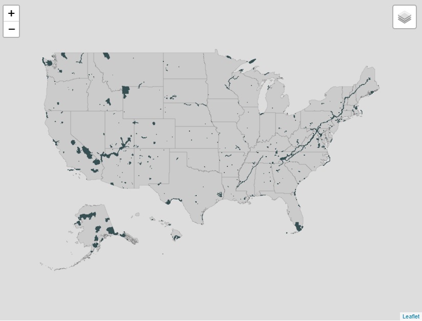
In this post, I will download and process the National Park data. Once that’s done, I’ll add it to the base map I created in part II.

project outline

I had to break the tutorial into different parts because it became unwieldy. I list the component parts below. The annotated version of the code can be found in this project’s repository in the folder called r files

I. cartography in r part one

• install packages
• download usa shapefile
• shift alaska and hawaii
• save shapefile

II. cartography in r part two

• create usa base map

III. cartography in r part three

• download national park data
• process national park data
• shift alaska and hawaii national parks
• save shapefile
• add national parks to map

IV. cartography in r part four

• download state park data
• process state park data
• shift alaska and hawaii state parks
• separate state park data
• save state park data

V. cartography in r part five

• add in shiny functionality
• add markers to visited parks
• save and embed map

VI. cartography in r part six

• create individual state maps
• add in shiny functionality
• add markers to visited parks
• save and embed maps

1. load libraries

1
2
3
4
5
    ## load libraries
    library("tidyverse")        # data manipulation & map creation
    library("sf")               # loads shapefile
    library("leaflet")          # creates the map
    library("operator.tools")   # not-in function

I am not going to explain in detail what each of these packages do because I already covered it in part one.

2. load usa data

1
2
    ## load data
    states <- read_sf("~/Documents/Github/nps/shapefiles/shifted/usa/usa.shp")

Be sure to change ~/Documents/Github/nps/shapefiles/shifted/usa/usa.shp to reflect wherever you saved the shifted shapefile.

If your data processing and base map creation are in the same file, you can skip this line, and when you make the Leaflet call below, you’ll use the name of the variable where the shape data is stored.

3. download national park data

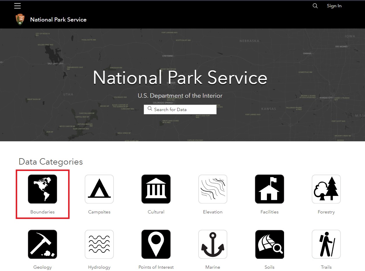
The National Park Service provides all the data we’ll need to make the map. The data is accessible on the ArcGIS’ Open Data website. Once you click on the link you’ll see a bunch of icons that lead to different data that’s available for download. Click on the one for boundaries.

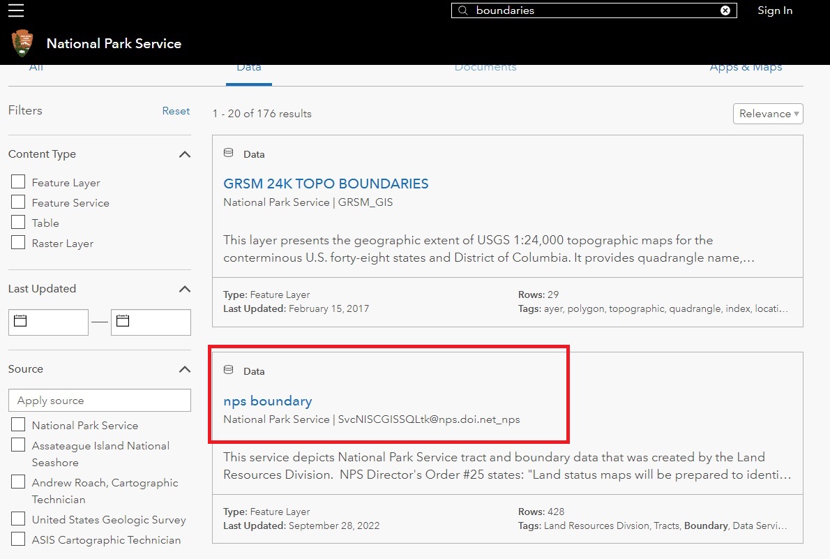
From here, you’ll be taken to a list of available National Park data. The second link should be nps boundary which contains the shape data for all the National Parks in the United States. The file contains all the data for the park outlines along with hiking trails, rest areas, and lots of other data.

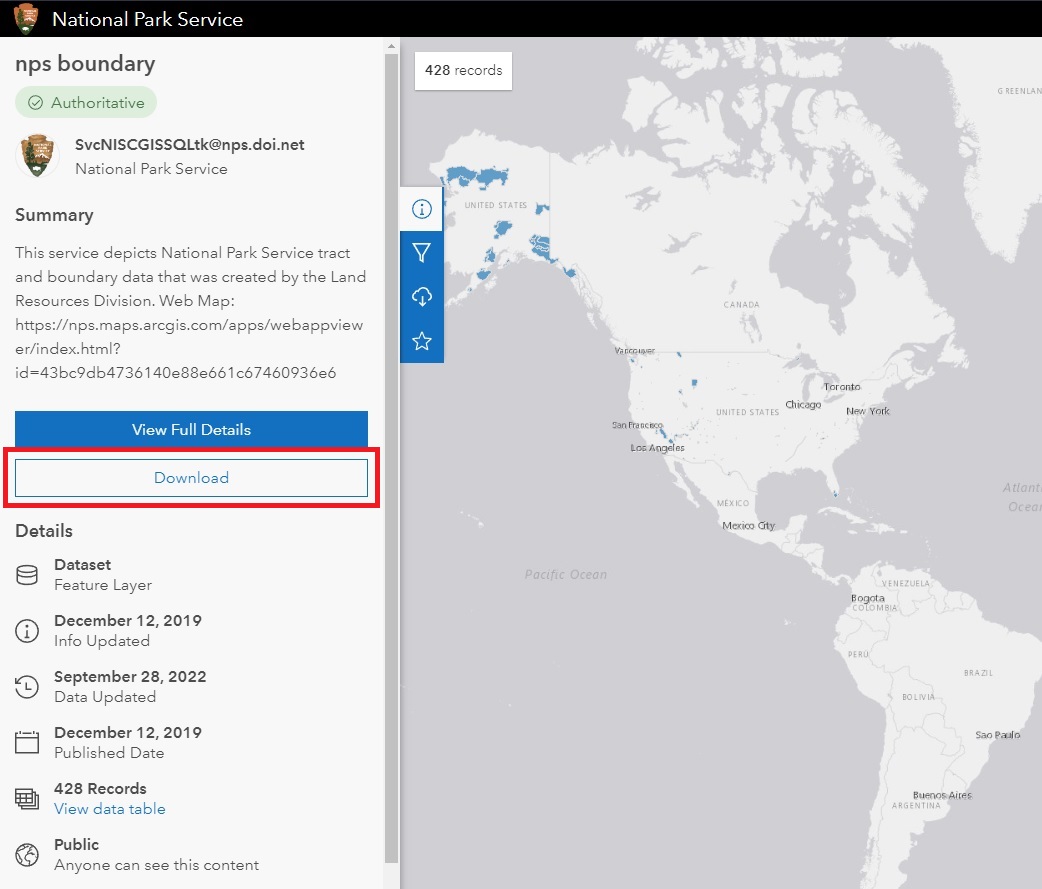
The nps boundary link will take you to a map showing the national parks. On the left, there will be a download link.

From here, you’ll have a few download options. The National Park Service provides the data in different formats including CSV and Shapefile. You’ll want to download the shapefile version.

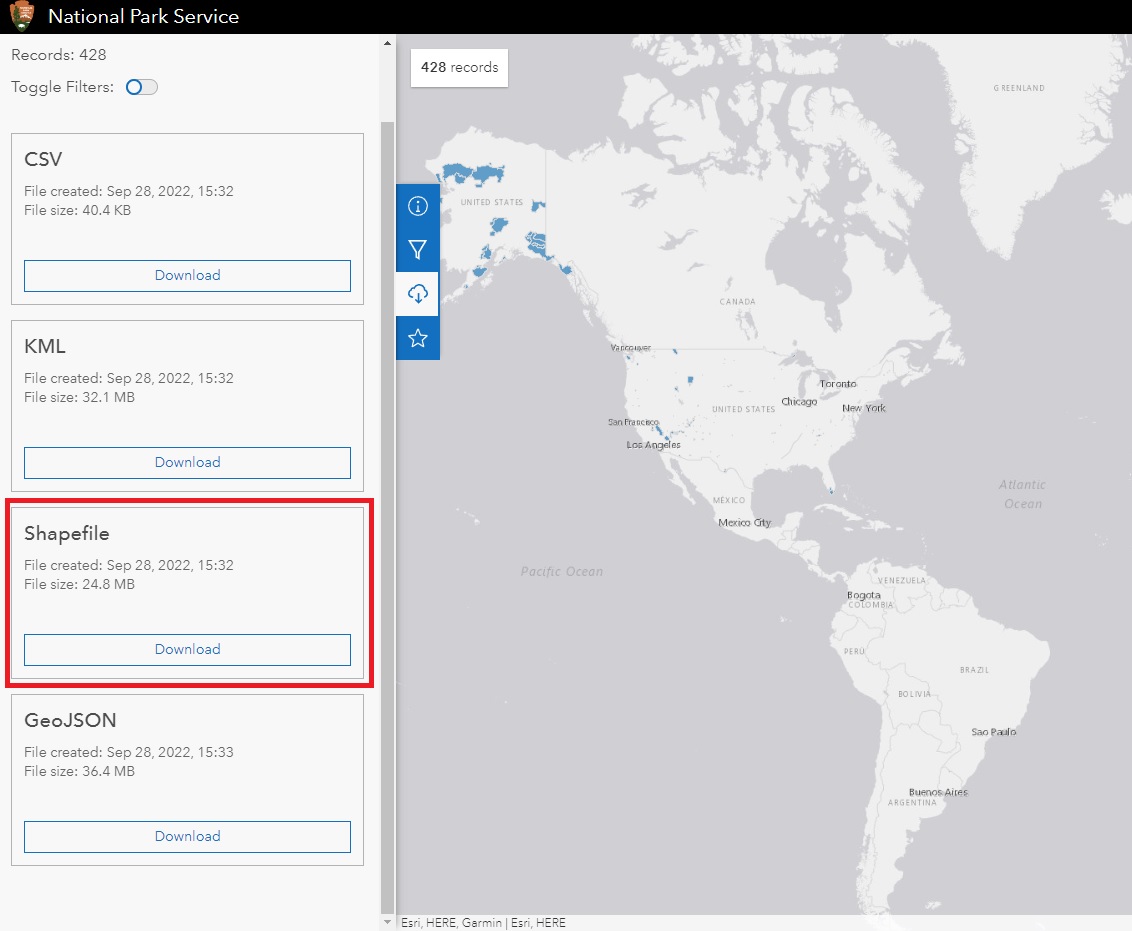
Be sure to save the file somewhere on your hard drive that is easy to find. When it finishes downloading, unzip the file. There will be four files inside the folder. All of them need to be kept in the same location. Although we’ll only load the .shp file, R uses the three others to create the necessary shapes.

4. process national park data

The code below may look intimidating, but it’s fairly straight forward. I’ll go over each line below.

1
2
3
4
5
6
7
8
9
10
11
12
13
14
15
16
17
18
19
20
21
22
23
24
25
26
27
28
29
30
31
32
33
34
35
36
37
38
39
40
41
42
43
    ## create territories list
    territories <- c("AS", "GU", "MP", "PR", "VI")

    ## load and process nps data
    nps <- read_sf("./shapefiles/original/nps/NPS_-_Land_Resources_Division_Boundary_and_Tract_Data_Service.shp")  %>% 
    select(STATE, UNIT_TYPE, PARKNAME, Shape__Are, geometry) %>% 
    filter(STATE %!in% territories) %>%  
    mutate(type = case_when(UNIT_TYPE == "International Historic Site" ~ "International Historic Site", # there's 23 types of national park, I wanted to reduce this number.
                UNIT_TYPE == "National Battlefield Site" ~ "National Military or Battlefield", # lines 56-77 reduce the number of park types
                UNIT_TYPE == "National Military Park" ~ "National Military or Battlefield", 
                UNIT_TYPE == "National Battlefield" ~ "National Military or Battlefield",
                UNIT_TYPE == "National Historical Park" ~ "National Historical Park, Site, Monument, or Memorial",
                UNIT_TYPE == "National Historic Site" ~ "National Historical Park, Site, Monument, or Memorial",
                UNIT_TYPE == "National Historic Trail" ~ "National Historical Park, Site, Monument, or Memorial",
                UNIT_TYPE == "National Memorial" ~ "National Historical Park, Site, Monument, or Memorial",
                UNIT_TYPE == "National Monument" ~ "National Historical Park, Site, Monument, or Memorial",
                UNIT_TYPE == "National Preserve" ~ "National Preserve, Reserve, or Recreation Area",
                UNIT_TYPE == "National Reserve" ~ "National Preserve, Reserve, or Recreation Area",
                UNIT_TYPE == "National Recreation Area" ~ "National Preserve, Reserve, or Recreation Area",
                UNIT_TYPE == "National River" ~ "National River, Lakeshore, or Seashore",
                UNIT_TYPE == "National Lakeshore" ~ "National River, Lakeshore, or Seashore",
                UNIT_TYPE == "National Wild & Scenic River" ~ "National River, Lakeshore, or Seashore",
                UNIT_TYPE == "National Seashore" ~ "National River, Lakeshore, or Seashore",
                UNIT_TYPE == "National Trails Syste" ~ "National Trail",
                UNIT_TYPE == "National Scenic Trail" ~ "National Trail",
                UNIT_TYPE == "National Park" ~ "National Park or Parkway",
                UNIT_TYPE == "Park" ~ "National Park or Parkway",
                UNIT_TYPE == "Parkway" ~ "National Park or Parkway",
                UNIT_TYPE == "Other Designation" ~ "Other National Land Area"))  %>%  
    mutate(visited = case_when(PARKNAME == "Joshua Tree" ~ "visited", 
                                PARKNAME == "Redwood" ~ "visited", 
                                PARKNAME == "Santa Monica Mountains" ~ "visited", 
                                PARKNAME == "Sequoia" ~ "visited", 
                                PARKNAME == "Kings Canyon" ~ "visited",
                                PARKNAME == "Lewis and Clark" ~ "visited",
                                PARKNAME == "Mount Rainier" ~ "visited",
                                TRUE ~ "not visited")) %>%  
    shift_geometry(preserve_area = FALSE, 
                    position = "below") %>% 
    sf::st_transform("+proj=longlat +ellps=WGS84 +datum=WGS84 +no_defs")

    ## save the shifted national park data
    st_write(nps, "~/Documents/GitHub/nps/shapefiles/shifted/nps/nps.shp")

• line 2

2    territories <- c("AS", "GU", "MP", "PR", "VI")

In part I of this series I talked about how R has an %in% function, but not a %!in% function. Here’s where the latter function shines.

The United States is still an empire with its associated territories and islands. In this project I am interested in the 50 states - without these other areas. As a result, I need to filter them out.

If i were to use base R’s %in% function, I would have to create a variable that contains the postal abbreviations for all 50 states. That is annoying. Instead, I want to use the shorter list that only includes the US’ associated islands and territories. To do so, however, I need to use the operator tools’ %!in% function. This means I can create a list of 5 postal codes rather than 50 of them.

Line 2 creates the list of US territories that I filter out in line 7. The c() function in R means combine or concatenate. Inside the parenthesis are the five postal codes for the American Samoa, Guam, the Northern Mariana Islands, Puerto Rico, and the Virgin Islands.

• line 5

5   nps <- read_sf("path/to/file/NPS_-_Land_Resources_Division_Boundary_and_Tract_Data_Service.shp")  %>% 

nps <- read_sf("path/to/file.shp") loads the National Park data set to a variable called nps using the read_sf() function that is part of the sf package. You will need to change the file path so it reflects where you saved the data on your hard drive.

The filename NPS_-_Land_Resources_Division_Boundary_and_Tract_Data_Service.shp will be the same. If you need help locating the filepath here is how to do it on a Mac and here is how to do it on Windows.

The %>% operator is part of the tidyverse package. It tells R to go to the next line and process the next command. The >%> has to go at the end of a line, rather than the beginning.

• line 6

6    select(STATE, UNIT_TYPE, PARKNAME, Shape__Are, geometry) %>%

select is part of the tidyverse package. It’s useful because we can select columns by their names (e.g. STATE) rather than their column number (e.g. STATE is column 12 in the original data set).

Each column in a data frame is automatically given an index number starting from 1 which can be used to select the column. For example, to select the STATE column by its number the code would be: state_only <- nps[,12].

The format is fairly simple. We assign the data to a variable state_only <- . Then R looks at the nps data set and picks out the data listed inside the square brackets. Inside the square brackets the value before the comma is the row number and the value after the comma is the column number. Here, I want all the rows for column 12 so I’ll leave the space before the comma empty.

Another example, if I wanted to choose the NPS data from rows 5 and 6 in column 12 it would be: nps[c(5,6),12]. This will return two rows (5 & 6) from one column (12)

Since I’m not a computer, I like to use the names so when I return to the code later I know exactly what I’m selecting without having to run extra code. To use the names, I use select from the tidyverse package.

If you want to learn more about selecting data here is how you can select columns using different methods in R.

The NPS data set has 23 columns, most of which I won’t use for this map. Select offers a way to pick out only the columns that I’ll need going forward. One reason for this is that large data sets take more computing power. The computer has to load more rows in more columns and then iterate over them. This causes the data processing and map rendering to be very, very slow.

Deciding on which columns to keep will depend on the data you’re using and what you want to map (or analyze). I know for my project I want to include a few things:

• the state where the park is located
• the park name
• the park type (park, battlefield, memorial, etc)
• and the park’s size.

There’s a couple ways to inspect the data to see what kind of information is available.

1. You can view the entire data set by using view(nps) but as the number of data points increases, so does R’s struggle with opening it. I’ve found that VSCode doesn’t throw as big of a fit as R Studio when opening large data sets.
2. Another way is to just look at the column names using data.frame(colnames(nps)). This will return a list of the data set’s column names. This is my preferred method. I then go to the documentation to see what each column contains. This isn’t fool-proof because it really depends on if the data has good documentation.

The National Park data includes a lot of information about who created the data and maintains the property. I’m not interested in this, so in line 6 I select the following columns:

• STATE [the two character state abbreviation]
• UNIT_TYPE [if it’s a national park, battlefield, etc]
• PARKNAME [the name of the park]
• Shape__Are [the size of the park]
• geometry

The geometry column is specific to shapefiles and it includes the coordinates of the shape. It will be kept automatically - unless you use the st_drop_geometry() function. I like to specifically select so I remember it’s there.

• line 7

7    filter(STATE %!in% territories) %>%  

In line 7 I use the territories list I created in line 2 to filter out the United States’ associated areas. Since the nps data uses the two character state abbreviation, I have to use the two character abbreviation for the territories. Searching for “Guam,” for example, won’t work.

filter() is part of the tidyverse and it uses conditional language. In the parentheses is a condition that must be true if the tidyverse is going to keep the row. Starting at the top of the data, R goes “alright, does the value in the STATE column match any of the values in the territories list?” If the condition is TRUE, R adds the row to the new data frame.

For example, if the STATE value in row 1 is CA, filter looks at it and goes “is CA NOT IN territories?” If that is TRUE, keep it because we want only the values that are NOT IN the territories list.

• lines 8-29

8    mutate(type = case_when(UNIT_TYPE == "International Historic Site" ~ "International Historic Site",

mutate() is part of the tidyverse package and it’s extremely versatile. It is mainly used to create new variables or modify existing ones.

The NPS data set has 23 different types of National Parks listed (you can view all of them by running levels(as.factor(nps$UNIT_TYPE))). I know that in later posts, I’m going to color code the land by type (blue for rivers, green for national parks, etc) so I wanted to reduce the number of colors I will have to use.

mutate()’s first argument, type = creates a new column called type. R will populate the newly created column with whatever comes after the first (singular) equal = sign. For example, I can put type = NA and every row in the type column will say NA.

Here, I am using the case_when() function, which is also part of the tidyverse. The logic of case_when is fairly straight forward. The first value is the name of the column you want R to look in (here: UNIT_TYPE). Next, is a conditional. I am looking for an exact match (==) to the string (words) inside the first set of quotation marks (in line 8: "International Historic Site").

The last part of the argument (after the tilde ~) is what I want R to put in the type column when it finds a row where the UNIT_TYPE is "International Historic Site". I want to keep historic sites in their own category for my map, so in line 8 I am telling R “If it’s an international historic site originally, populate this new column with that information.”

In lines 9-12 you can see how I use case_when() to reduce the number of park types. I combine Military Parks, Battlefields, and Battlefield Sites into one catch-all term “National Military or Battlefield”.

In its general form, the format is case_when(COLUMN_NAME == "original_value" ~ "new_value")

Lines 9-29 do the same thing for the other park types. You can reduce the parks however you want or use all 23 types. Just remember that the value before the tilde ~ has to match the values found in the data exactly. For example, in line 24 I change the NPS data’s National Trail Syste value to be National Trail. However the data was created, System in this case is missing the m.

• lines 30-37

30    mutate(visited = case_when(PARKNAME == "Joshua Tree" ~ "visited",

Lines 30-37 use the same mutate() and case_when logic as above. Instead of reducing the number of park types, I use it to mark the different parks I have visited.

Line 30 creates the new column, visited and uses case_when to look for the names of the parks that I’ve been to. If I have visited them, it adds visited to the column of the same name.

The last line, TRUE ~ "not_visited")), acts as an else statement. For any park not listed above, it will put not visited in the visited column I created.

This feels like a very brute-force method of tracking which parks I’ve visited, but I haven’t spend much time trying to find another way.

• line 38-39

38    shift_geometry(preserve_area = FALSE, 
39                   position = "below") %>%

In part I, when I made the base map, I moved Alaska and Hawaii so they were of similar size and closer to the continental USA. For the map to display the parks correctly, I have to shift them as well.

I went over these two lines in part II, so I won’t go over them again here. If you want to read more about them, check out that post.

• line 40

40  sf::st_transform('+proj=longlat +datum=WGS84')

The last line uses the st_transform() function from the sf package to covert the data set from NAD83 to WGS84. Leaflet requires WGS84, so be sure to include this line at the end of your data manipulation.

I covered the WGS84 ellipsoid in part I, if you want to read more about it.

• line 43

43  st_write(nps, "~/Documents/GitHub/nps/shapefiles/shifted/nps/nps.shp")

Strictly speaking, you don’t need to save the changes to a new shapefile using this line. You can do all your data processing in the same file where you make your map, but I prefer to separate the steps into different files.

As a result, I save the shifted data to my hard drive so it’s easier to load later. I usually have this line commented out (by placing # at the start of the line) after I save it the first time. I don’t want it to save every time I run the rest of the code.

5. add national parks to base map

1
2
3
4
5
6
7
8
9
10
11
12
13
14
15
16
17
18
19
20
21
22
23
24
25
26
27
28
29
30
31
32
33
34
    ## add National Parks to USA Base Map using leaflet()
    map <- leaflet() %>%
    addPolygons(data = states,
        smoothFactor = 0.2,
        fillColor = "#808080",
        fillOpacity = 0.5,
        stroke = TRUE,
        weight = 0.5,
        opacity = 0.5,
        color = "#808080",
        highlight = highlightOptions(
            weight = 0.5,
            color = "#000000",
            fillOpacity = 0.7,
            bringToFront = FALSE),
        group = "Base Map")  %>% 
    addPolygons(data = nps,
        smoothFactor = 0.2,                 
        fillColor = "#354f52",
        fillOpacity = 1,
        stroke = TRUE,
        weight = 1,     
        opacity = 0.5,                       
        color = "#354f52",             
        highlight = highlightOptions(
            weight = 3,
            color = "#fff",
            fillOpacity = 0.8,
            bringToFront = TRUE),
        group = "National Parks")  %>%
    addLayersControl(
        baseGroups = "Base Map",
        overlayGroups = "National Parks",
        options = layersControlOptions(collapsed = FALSE))

• lines 2-16

Lines 2-16 are identical to those in part II where I created the base map. I am not going to cover these sections in detail, because I covered it previously.

• line 17

17    addPolygons(data = nps,

To add the National Park data to the base map, we call addPolygons() again. The arguments are the same as before - color, opacity, outline style - just with different values. By changing those values, we can differentiate the base map from the national park data.

Since we’re mapping the National Parks and not the states, we have to tell R where the data is located using data = nps.

nps is the variable name where the shape data is stored. It will change based on what you named your data.

• line 18

18   smoothFactor = 0.2,

smoothFactor() determines how detailed the park boundaries should be. The lower the number, the more detailed the shape. The higher the number, the smoother the parks will render. I usually match this to whatever I set for the base map for consistency.

• lines 19-20

19   fillColor = "#354f52",
20   fillOpacity = 1,

Define the color and transparency of the National Parks. In a future post, I am going to change the color of each type of public land, but for now, I’ll make them all a nice sage green color #354f52. I also want to make the parks fully opaque by setting the fillOpacity=1.

• lines 21-24

21    stroke = TRUE,
22    weight = 1,     
23    opacity = 0.5,                       
24    color = "#354f52",

The next four lines (21-24) define what kind of outline the National Parks will have. I detail each of these arguments in part II of this series.

Briefly, I want there to be an outline to each park (stroke = TRUE) that’s thicker weight = 1 than the outline used on the base map. I do not like the way it looks at full opacity, so I make it half-transparent (opacity = 0.5). Finally, I want the outline color = "#354f52" to be the same color as the fill. This will matter more when I change the fill color of the parks later on.

• lines 25-28

25  highlight = highlightOptions(
26              weight = 3,
27              color = "#fff",
28              fillOpacity = 0.8,

Lines 25-28 define the National Park’s behavior on mouseover. First we have to define and initialize the highlightOptions() function. The function take similar arguments as the addPolygons function - both of which I go over in detail in part II.

I want to keep the mouseover behavior noticeable, but simple. To do so, I set the outline’s thickness to be weight = 3. This will give the shape a nice border that differentiates it from the rest of the map.

color = "#fff" sets the outline’s color on mouseover only. So, when inactive, the outline color will match the fill color, but on mouseover the outline color switches to white (#fff).

• line 29

29    bringToFront = TRUE),

bringToFront can either be TRUE or FALSE. If TRUE, Leaflet will bring the park to the forefront on mouseover. This is useful later when we add in the state parks because national and state parks tend to be close together.

When FALSE the shape will remain static.

• line 30

30    group = "National Parks")  %>%

Since Leaflet adds all new data to the top of the base map, I think it’s useful to group the layers together. In the next block of code, we add in some layer functionality. For now, though, I want to add the National Parks to their own group so I can hide the National Parks if I want.

• line 31-34

31    addLayersControl(
32        baseGroups = "Base Map",
33        overlayGroups = "National Parks",
34        options = layersControlOptions(collapsed = FALSE))

addLayersControl defines how layers are displayed on the final map. The function takes three arguments.

First, we have to tell Leaflet which layer should be used as the base map: baseGroups = "Base Map". The name in the quotations (here: "Base Map") has to match the name given to the layer you set in the addPolygons() call. In line 14, I put the 50 states into a group called "Base Map", but you can name it anything you like.

There can be more than one base map, too. It’s not super helpful here since I shifted Alaska and Hawaii, but when using map tiles you can add multiple types of base maps that users can switch between.

Next, we have to define the layers that are shown on top of the base group: overlayGroups = "National Parks". Just like the base map, this is defined in the corresponding addPolygons call. Here, I called the layer National Parks in line 30.

Finally, on the map I don’t want the layers to be collapsed, so I set options = layersControlOptions(collapsed = FALSE). When TRUE the map will display an icon in the top right that, when clicked, will show the available layers (see image below).

6. conclusion

Hey, look at that! You made a base map and you added some National Park data to it. You’re a certified cartographer now!

In the next part IV post we’ll download and process the state park data before adding it to the map. Part V of this series we’ll add Shiny functionality and some additional markers.