cartography in R part one

Twitter is a great resource for engaging with the academic community. For example, I saw this Tweet by PhD Genie asking users to name one positive skill learned during their PhD. I love this question for a number of reasons. First, it helps PhDs reframe their experience so it’s applicable outside of academia - which can help when applying to jobs. Second, it’s really cool to see what skills other people have learned during their program.

I responded to the tweet because during my PhD I learned how to create maps in R. I started by recreating a map from the University of North Carolina’s Hussman School of Journalism’s News Deserts project (below). Now, I am working on a personal project mapping the U.S. National and State parks.

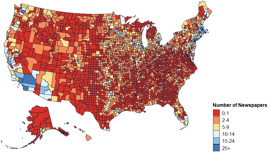
There was quite a bit of interest in how to do this, so in this series of posts I will document my process from start to finish.

a few notes

First, I’m not an expert. I wanted to make a map, so I learned how. There may be easier ways and, if I learn how to do them, I’ll write another post.

Second, before starting, I strongly suggest setting up a Github and DVC. I wrote about how to use GitHub, the Github Website, and Github Desktop in a different series of posts. You can use any of these methods to manage your repositories. I use all three based purely on whatever mood I’m in.

If you do use Git or GitHub, then DVC (data version control) is mandatory. GitHub will warn you that your file is too large if it’s over 50MB and reject your pushes if the files are over 100MB. The total repository size can’t exceed 2GB if you’re using the free version (which I am).

DVC is useful because cartography files are large. They contain a lot of coordinates which increases with each location you try to map. DVC will store your data outside of GitHub but allows you to track changes with your data. It’s super useful.

Third, there are several ways to make a map. R is capable of making static and interactive maps. Static maps are less computationally expensive and better for publication. Interactive maps are prettier and better for displaying on the web.

I make interactive maps with Leaflet and Shiny because they offer a lot of functionality. The most common way is to use map tiles. Map tiles use data from sources like Open Street Map and Maps to create map squares (tiles) with custom data on top. A list of available map tiles can be found on the Open Street Maps website.

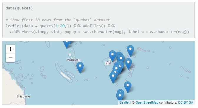
When I make static maps (like the US map pictured above), I use ggplot.

project outline

I had to break the tutorial into different parts because it became unwieldy. I list the component parts below. The annotated version of the code can be found in this project’s repository in the folder called r files

I. cartography in r part one

• install packages
• download usa shapefile
• shift alaska and hawaii
• save shapefile

II. cartography in r part two

• create usa base map

III. cartography in r part three

• download national park data
• process national park data
• shift alaska and hawaii national parks
• save shapefile
• add national parks to map

IV. cartography in r part four

• download state park data
• process state park data
• shift alaska and hawaii state parks
• separate state park data
• save state park data

V. cartography in r part five

• add in shiny functionality
• add markers to visited parks
• save and embed map

VI. cartography in r part six

• create individual state maps
• add in shiny functionality
• add markers to visited parks
• save and embed maps

1. install packages

You only need to install the packages once. You can do so by running each line in the terminal. When you rerun the code later, you can skip right to loading the packages using library("package-name")

1
2
3
4
5
6
7
8
    ## you only need to install the packages once

    install.packages("leaflet")        # interactive maps
    install.packages("shiny")          # added map functionality
    install.packages("tidyverse")      # data manipulation
    install.packages("tigris")         # cartographic boundaries
    install.packages("operator.tools") # for the not-in function
    install.packages("sf")             # read and write shapefiles

package descriptions

3    install.packages("leaflet")

• Leaflet is an open source mapping library used to create interactive maps. All leaflet maps have the same basic components:
  • A map widget (created by calling leaflet())
  • Layers (or features) added using addTiles(), addPolygons(), or addMarkers().
    
    Leaflet was originally written in Javascript by “Volodymyr Agafonkin, a Ukrainian citizen living in Kyiv.” With the Russian invasion of Ukraine, Volodymyr, his family, and the people he knows are being forced to flee. If you can, make a donation to Come Back Alive or to one of the charities listed at Stand With Ukraine. If you think the invasion is justified, don’t forget to carry some seeds in your pocket

4    install.packages("shiny")

• Shiny is an R package that provides additional functionality. I am primarily using it to create an informative tool box so the map is not overwhelmed by using too many popups.

5    install.packages("tidyverse")

• The Tidyverse is a collection of packages used for data manipulation and analysis. Its syntax is more intuitive than base R. Furthermore, you can chain (aka pipe) commands together.

  For cartography, you don’t need the whole Tidyverse. We’ll mainly use dplyr and ggplot. You can install these packages individually instead of installing the whole tidyverse. Though, when we get to the national park database, we’ll also need purr and tidyr.

6    install.packages("tigris")

• Tigris is used to load Census data and shapefiles. You can download the same data from the Census website, but it’s nice that you can do it in R.

7    install.packages("operator.tools")

• operator.tools is not required, but it’s recommended.

  For some unknown reason, base R has a %in% function but not a not-in function. Unfortunately, the United States is still an empire with its associated areas, islands, and pseudo-states. I only want to include the 50 states, so I needed a way to easily filter out the non-states. Operator tool’s %!in% function is perfect for that.

8    install.packages("sf")

• sf is used to read and write the shapefiles necessary for cartography.

2. load the packages

To start, create and save a new file called usa.r. In it, we’re going to download and modify the United States shape data that we’ll use to create the base map in part two of this series.

At the beginning of each file, you have to load the necessary packages. In this file, the only packages we need to load are tidyverse, sf, and tigris. I also load leaflet to make sure the map renders correctly.

1
2
3
4
5
    ## load libraries
    library("tidyverse")
    library("sf")
    library("tigris")
    library("leaflet")

3. download usa shapefile

There’s two ways to download the USA shape data. First, we can use the R package, tigris. Second, we can download it from the Census website.

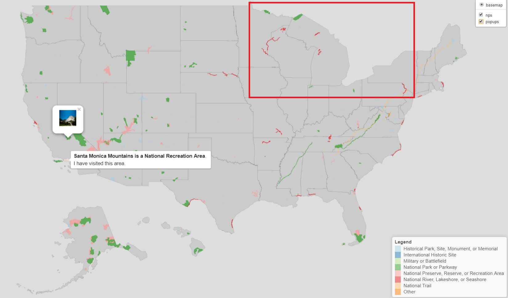
I prefer using tigris but I’ve been having some problems with it. Sometimes it ignores the Great Lakes and merges Michigan and Wisconsin into a Frankenstate (boxed in red below).

method 1: using tigris()

tigris() downloads the TIGER/Shapefile data directly from the Census and includes a treasure trove of data. Some of the data includes land area, water area, state names, and geometry.

Tigris can also download boundaries for counties, divisions, regions, tracts, blocks, congressional and school districts, and a whole host of other groupings. A complete list of available data can be found on the packages’ GitHub.

1
2
3
4
5
6
7
8
9
    ## download state data using tigris()
    us_states <- tigris::states(cb = FALSE, year = 2020)  %>% 
        filter(STATEFP < 57)  %>% 
        shift_geometry(preserve_area = FALSE,
                       position = "below")  %>% 
        sf::st_transform("+proj=longlat +ellps=WGS84 +datum=WGS84 +no_defs")
    
    ## save the shifted shapefile
    st_write(us_states, "path/to/file/usa.shp")

Here we create the us_states variable, save the geographic data to it, move Alaska and Hawaii so they’re beneath the continental US, and save the shifted shapefile.

• line 2:

2   us_states <- tigris::states(cb = FALSE, year = 2020)  %>%

R uses the <- operator to define new variables. Here, we’re naming our new variable us_states.

In our us_states variable we’re going to store data on the 50 states downloaded using tigris. Within (::) tigris, we’re going to use the states() function.

The states() function allows you to pull state-level data from the Census. This function takes several arguments.

The cb argument can either be TRUE or FALSE. If cb = FALSE tells Tigris() to download the most detailed shapefile. If cb = TRUE it will download a generalized (1:5000k) file. After a lot of trial and error, I found that using cb = TRUE prevents the Frankenstate from happening.

If the year argument is omitted it will download the shapefile for the default year (currently 2020). I set out of habit because I do work at the county level and county boundaries change more than state boundaries.

Finally, the %>% operator is part of the Tidyverse. It basically tells R “Hey! I’m not done, keep going to the next line!”

• line 3:

3    filter(STATEFP < 57)  %>% 

tigris::states() downloads data for the 50 states and the United States’ minor outlying islands, Puerto Rico, and its associated territories. Each state and territory is assigned a unique two-digit Federal Information Processing Standard [FIPS] code.

They’re mostly consecutive (Alaska is 01) but when they were conceived of in the 1970s a couple were reserved for the US territories (American Samoa was 03), but in the updated version the “reserved codes” were left out and the territories were assigned to new numbers (American Samoa is now 60). The important bit about this is that the last official state (Wyoming) has a FIPS of 56.

This line of code uses the filter() function on the STATEFP variable downloaded using Tigris(). All it says is keep any row that has a FIPS of less than 57. This will keep only the 50 states and exclude the United States’ empire associated territories.

• lines 4-5:

4    shift_geometry(preserve_area = FALSE,
5                   position = "below")  %>%

The shift_geometry() is from the Tigris package. It takes two arguments preserve_area and position.

When preserve_area = FALSE tigris will shrink Alaska’s size and increase Hawaii’s so that they are comparable to the size of the other states.

The position argument can either be "below" or "outside". When it’s below, both Alaska and Hawaii are moved to be below California. When it’s outside then Alaska is moved to be near Washington and Hawaii is moved to be near California.

Since I’m a born-theorist, I should warn you that messing with maps has inherent normative implications. The most common projection is Mercator which stretches the continents near the poles and squishes the ones near the equator.

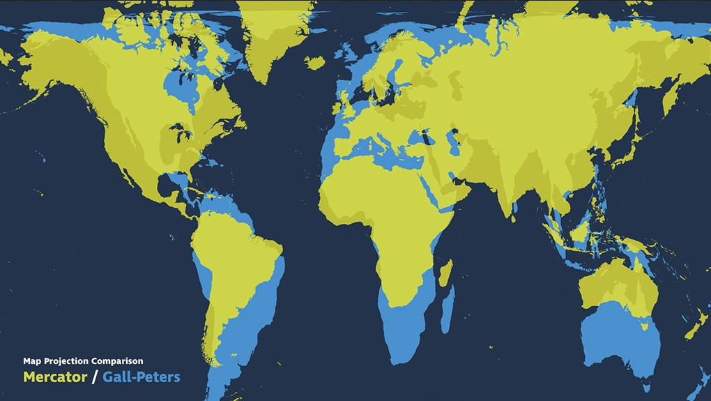
One of the competing projections is Gall-Peters which claims to be more accurate because it was - at the time it was created in the 1980s - the only “area-correct map.” Though it has now been criticized for skewing the polar continents and the equatorial ones. The above photo shows you just how different the projects are from one another.

The problem arises because we’re trying to project a 3D object into 2D space. It’s a classic case of even though we can, maybe we shouldn’t. Computers can do these computations and change the projections to anything we want fairly easily. However, humans think and exist in metaphors. We assume bigger = better and up = good. When we project maps that puts the Northern Hemisphere as both upwards and larger than other parts of the world we are imbuing that projection with metaphorical meaning.

I caution you to be careful when creating maps. Think through the implications of something as simple as making Alaska more visually appealing by distorting it to be of similar size as the other states.

If you want to read more about map projections this is a good post. If you want to read more about metaphors, I suggest Metaphors We Live By by George Lakoff and Mark Johnson.

• line 6:

6    sf::st_transform("+proj=longlat +ellps=WGS84 +datum=WGS84 +no_defs")

The sf package includes a function called st_transform() which will reproject the data for us. There are a lot of projections. You can read them at the proj website.

Leaflet requires all boundaries use the World Geodetic Service 1984 (WGS84) coordinate system. While making maps I’ve come across two main coordinate systems: WGS84 and North American Datum (1983). WGS84 uses the WGS84 ellipsoid and NAD83 uses the Geodetic Reference System (GRS80). From what I’ve gathered, the differences are slight, but leaflet requires WGS and the Census uses NAD83. As a result, we have to reproject the the data in order to make our map.

The st_transform function takes four arguments, each preceded by a +. All four arguments are required to transform the data from NAD83 to WGS84.

Briefly, +proj=longlat tells R to use project the code into longitude and latitude [rather than, for example, transverse mercator (tmerc)].

+ellps=WGS84 sets the ellipsoid to the WGS84 standard.

+datum=WGS84 is a holdover from previous proj releases. It tells R to use the WGS84 data.

+no_defs is also a holdover.

Essentially, you need to include line 6 before you create the map, but after you do any data manipulation. It might throw some warnings which you can just ignore.

• line 9

9    st_write(us_states, "path/to/file/usa.shp")

In the last line, we save the data we manipulated in lines 2-6. Strictly speaking you don’t have to save the shapefile. You can manipulate the data and then skip right to mapping the data. I caution against it because the files can get unreadable once you start using multiple data sets. I usually comment out line 9 after I save the file. That way I’m not saving and re-saving it whenever I need to run the code above it.

The st_write() function is part of the sf package and it takes two arguments. The first is the data set you want to save. Since I used us_states to save the data, it will be the first argument in the st_write() function call.

The second argument is the path to where you want the file saved and what name you want to give it. I named mine usa. It is mandatory that you add .shp to the end of the filepath so that R knows to save it as a shapefile.

Although it’s called a shapefile, it’s actually four files. I usually create a separate folder for each set of shapefiles and store that in one master folder called shapefiles. An example of my folder structure is below. I keep all of this in my GitHub repo and track changes using DVC.

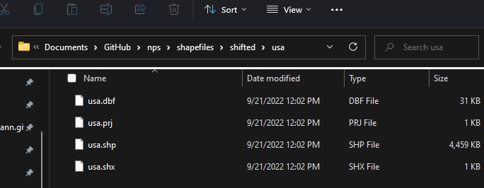
On my C:// drive is My Documents. In that folder I keep a GitHub folder that holds all my repos, including my nps one. Inside the nps folder I separate my shapefiles into their own folder. For this tutorial I am using original and shifted shapefiles, so I’ve also separated them into two separate folders to keep things neat. I also know I’m going to have multiple shapefiles (one for the USA, one for the National Parks, and a final one for the State Parks) so I created a folder for each set. In the usa folder I saved the shifted states shapefile.

Altogether, my line 9 would read:

9    st_write(us_states, "~/Documents/GitHub/nps/shapefiles/shifted/usa/usa.shp")

Running that line will save the four necessary files that R needs to load the geographic data.

That’s it for method 1 using tigris. The next section, method 2, shows how to load and transform a previously downloaded shapefile. If you used method 1, feel free to leave this post and go directly to mapping the shapefile in part II of this series.

method 2: using downloaded shapefiles

In this section, I’ll go through the process of downloading the shapefiles from the Census website. If you tried method 1 and tigris caused the weird Frankenstate, you can try using the data downloaded from the Census website. I don’t know why it works, since tigris uses the same data, but it does.

Generally, though, finding and using shapefiles created by others is a great way to create cool maps. There are thousands of shapefiles available, many from ArcGis’ Open Data Website.

• step 1:
  On the Census website, select the Data & Maps dropdown. In the dropdown, on the right-hand side you’ll select Mapping Files.

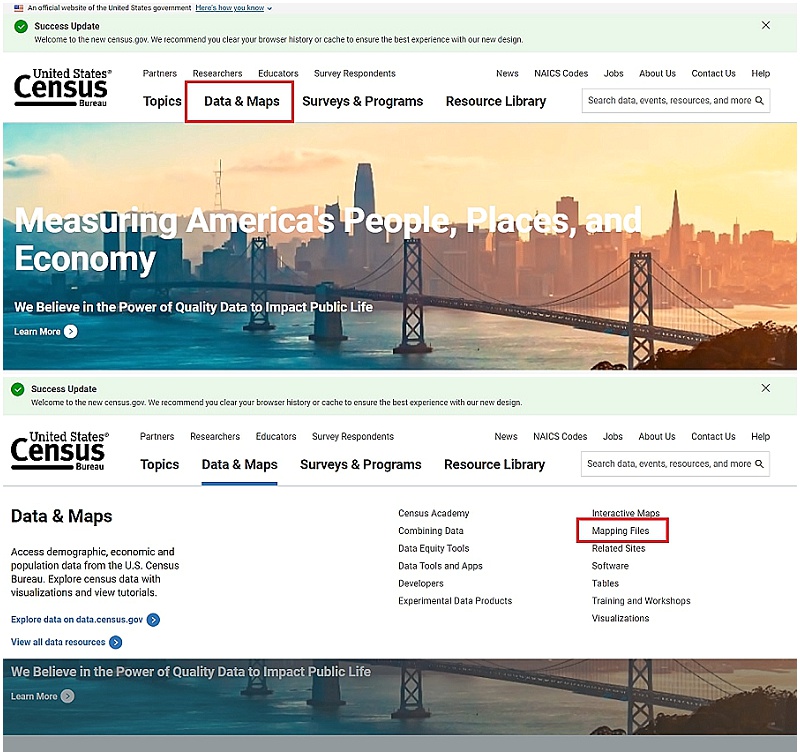
• step 2:
  From here, about halfway down on the page, there’s a link called TIGER Data Products Guide which will take you to a complete list of the shapefiles available.

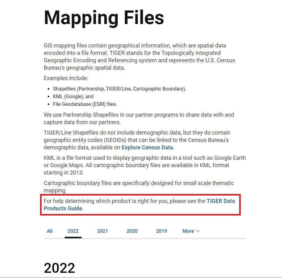
• step 3:
  There’s a lot of downloads available on this page, but for now just click on “Cartographic Boundaries Shapefiles.” Make sure you select the shapefiles one and not the Geodatabases or Geopackages link.

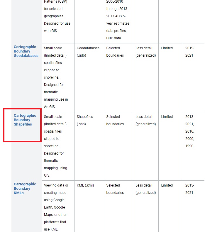
Save the file wherever you want, but I prefer to keep it within the “original” shapefiles folder in a sub-folder called “zips.” Once it downloads, unzip it - again, anywhere is fine. It will download all 30 Census shapefiles. We’re only going to use the one called “cb_2021_us_state_500k.zip”. The rest you can delete, if you want.

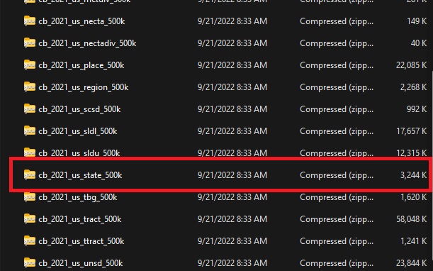
When you unzip the cb_2021_us_state_500k.zip, it will contain four files. You’ll only ever work with the .shp file, but the other three are used in the background to display the data.

• step 4:

Once all the files are unzipped, we can load the .shp file into R.

1
2
3
4
5
6
7
8
9
    ## load a previously downloaded shapefile
    usa <- read_sf("shapefiles/original/usa/states/cb_2021_us_state_500k.shp") %>%
        filter(STATEFP < 57) %>%
        shift_geometry(preserve_area = FALSE,
            position = "below") %>%
        sf::st_transform("+proj=longlat +ellps=WGS84 +datum=WGS84 +no_defs")

    ## save the shifted shapefile
    st_write(usa, "path/to/file/usa.shp")

Everything except line 2 is the same as in method 1. I won’t go over lines 3-9 here, because all the information is above.

• line 2:

This line is very similar to the one above. I changed the name of the variable to usa so I could keep both methods in the same R file (each R variable needs to be unique or it will be overwritten).

read_sf is part of the sf() package. It’s used to load shapefiles into R. The path to the file is enclosed in quotation marks and parentheses. Simply navigate to wherever you unzipped the cb_2021_us_state_500k file and choose the file with the .shp extension.

4. conclusion

Once the shapefiles are downloaded - either using tigris() or by loading the shapefiles from the Census website - you can create the base map. I’ll tackle making the base map in Part II of this series.